[Matlab] figure aspect ratio/print figure as it appears on the screen

 

Hi, Sisi is here! I decided to contribute to the journal club blog again. It's not that easy to get rid of me after all... I also decided to start my own blog at http://binarymumbles.blogspot.com/.
Now on to the bussiness.

If you use Matlab to plot some data (esp. time series data, say if your want to plot some behavior over a long period of time), you will likely encounter the following problem. Sometimes, the ratio of the figure just looks ugly. This post points out several ways to solve this problem. If you are in a hurry, just scroll down and read code snippet 4.

 try the following code:

% ========== code snippet 1 ==========
y=rand(2000,1); % generate 2000 random numbers
x=1:1:2000; % generate indices
plot(x,y,'color','k'); % plot
% ========== end of snippet ========== 


You will get something like this:

This figure will look more pleasing if it is stretched horizontally. To do that, we can add a statement that modify the size of the figure.

% ========== code snippet 2 ==========
y=rand(2000,1);
x=1:1:2000;
fig=figure; % create a figure handle
set(fig,'Position',[0 0 1000 200]); % change figure height to 2000 pixels and width to 200 pixels
plot(x,y,'color','k');
figname='fig1';
print(fig,'-dtiff',figname); % saving figure to tiff format 
% ========== end of snippet ========== 

This is how the figure look on the screen, x-axis is more stretched out, giving a better view. But if you look at the saved tiff file "fig1.tiff", you will find that the saved figure looks like the earlier figure, the one with a shorter x-axis. So, now the question is, how do we save the figure as it appears on the screen? After some internet search, I found out this easy hack for windows: simply save your figure in bitmap format instead of tiff (or other figure formats). Figures in bitmap format are displayed at screen resolution, therefore, saving as bitmap preserve the ratio.

% ========== code snippet 3 ==========
y=rand(2000,1);
x=1:1:2000;
fig=figure; % create a figure handle
set(fig,'Position',[0 0 1000 200]); % change figure height to 2000 and width to 200
plot(x,y,'color','k');
figname='fig2';
print(fig,'-dbitmap',figname); % saving figure to bitmap format 
% ========== end of snippet ========== 

However, this solution is suboptimal in several ways:
(1) It only work on windows.
(2) It is not ideal for printing high quality pictures. You can not get a figure that have more pixels than your screen resolution. (Change line 4 in code snipet 3 to set(fig,'Position',[0 0 10000 2000]); and check the height and width of the saved figure).

Is there a better way? Well, absolutely! Otherwise I will not be writing this post :)

% ========== code snippet 4 ==========
y=rand(2000,1);
x=1:1:2000;
fig=figure;
plot(x,y,'color','k');
daspect([500 1 1]); % change aspect ratio of x-y axis (in this example, the length of 500 unit on x axis equals 1 unit on y axis)
figname='fig3';
print(fig,'-dtiff','-r300',figname);
% ========== end of snippet ==========

Now everything is pretty!

Basics of Immunohistochemistry

Immunohistochemistry is the process of detecting and visualizing antigens using antibodies. In principle, antibodies can be raised against almost any type of antigen. For the present guide, we will focus on proteins, which are among the most common antigens detected.

To visualize the antigen, one must:

1) Collect and fix tissue
2) Section tissue
3) Antigen Retrieval (if necessary)
4) Block Endogenous Enzymes
5) Incubate with a Primary Antibody
6) Incubate with a Secondary Antibody
7) Reveal the reaction with a reporter molecule


Lets explore these steps a little more:

1) Collecting and fixing tissue involves removing the desired tissue and using a chemical agent to preserve the tissue from decay.  In immunohistochemistry, paraformaldehyde  is often used to fix tissue because paraformaldehyde creates cross-links between proteins. Besides instilling mechanical stability in the tissue, it is also believed that the cross-links between proteins serve to trap other molecules that may be of interest (e.g. nucleic acids).

2) Sectioning tissue can be accomplished using a number of different methods. Common techniques involve embedding tissue in paraffin blocks, or embedding tissue in a freezing medium before slicing the tissue. When conducting frozen sectioning, it is often necessary to cryo-protect the tissue prior to sectioning. Sucrose is used as a common cryo-protectant as it is able to partially dehydrate tissue and prevent the formation of ice-crystals as the tissue freezes. Tissue is typically left in a 20-30% sucrose solution until the specific gravity of the tissue and the solution are approximately in balance, causing the tissue to sink. Sectioning then involves freezing the tissue by surrounding it with OCT or another freezing medium and using the freezing components of a microtome of cryostat to slowly freeze the tissue. A steel knife mounted on the sectioning apparatus is then used to repeatedly cut sections of a desired thickness.

3) For some staining techniques, antigen retrieval is necessary or can improve the quality of staining.  This process involves specialized reagents that can break the protein cross-links that have been formed by paraformaldehyde (or other fixatives) and uncovering biding sites that might have been hidden by these cross-links.

4) Endogenous peroxidases can exist in many cells or tissues. If present, peroxidases can result in a large amount of background staining that will not be specific to the antigen of interest.  One can test for the presence of endogenous peroxidase activity by incubating tissue with a DAB solution.  If the tissue turns brown, then the tissue contains endogenous peroxidase that that must be blocked.  Typically this type of blocking is done by exposing the tissue to a hydrogen peroxide solution. This reaction causes the irreversible inactivation of endogenous perodidase.

It is also necessary to ensure that the antibody for one's target antigen does not bind to non-specific binding sites.  To do this, these non-specific binding sites are saturated using a blocking agent.  Blocking agents like goat serum or BSA bind to portions of tissue with a net positive charge or portions that are hydrophobic. Without blocking, these areas would also serve to attract and bind most primary and secondary antibodies.

5) The next step in staining for a specific antigen is to incubate the tissue in the primary antibody.  This is as simple as diluting the antibody to a specific concentration and then allowing the tissue to agitate for a specified period in order to allow the primary antibody sufficient time to bind to the antigen sites.

One common question related to this form of blocking is how it is possible to block all of the non-specific sites on tissue and not block binding sites for our antigen of interest. The answer to this is actually quite simple: blocking buffers do in fact block antigen binding sites, but the types of bonds formed by the blocking buffer are very weak and can easily be reversed. Therefore, the high antibody-antigen affinity will always prevail over the bond between the blocking buffer and the antigen.

6) Similar to incubation of the primary antibody, tissue subsequently needs to be incubated with the secondary antibody. The secondary antibody is designed to bind to the primary antibody. Generally, this is accomplished by creating a secondary antibody that has been raised against immunoglobulin (IgG) for the species from which the primary antibody was derived.

7) The final step in an immunohistochemistry protocol is generally to reveal the antigen binding sites using a reporter molecule.  For fluorescent IHC, it is often the case that a fluorescent tag will be incorporated with the secondary antibody. Alternatively, signals can be further amplified by binding biotin molecules or an avidin-biotin peroxidase complex. The peroxidase in the complex is then revealed using DAB (3,3'-Diaminobenzidine). The oxidation of peroxidase using DAB and H202 results in formation of a free radical intermediate which polymerizes to form a brown stain. This reaction can also be turned black via the addition of Nickel to the reaction.

Hopefully this helps you to understand the steps involved in IHC. good luck staining!

D.J. Barker

Acoustics: Stimulus Presentation in the rat

There are a number of things to consider when presenting auditory stimuli to laboratory animals. One thing that we must not forget is that auditory stimuli are perceived differently by rodents than they are by humans. Thus, if we present a relatively low frequency tone to an animal, it is likely that their perception is different than the perception of the experimenter setting its intensity. As you can see from the collection of audiograms below (Engle & Barnes, 2012), stimuli below 1 kHz quickly fall outside of rats' hearing range but are still near the optimal range for humans.

Knowing this, imagine if you were to associate a 500 Hz tone with food delivery and a 2 kHz tone with sucrose delivery in a Pavlovian paradigm. Can you guarantee that the increased rate of approach for sucrose is in fact related to the increased incentive salience for that reward? Hopefully you would have learned about counterbalancing long before this, but if not, you can see how you might have a problem on your hands.

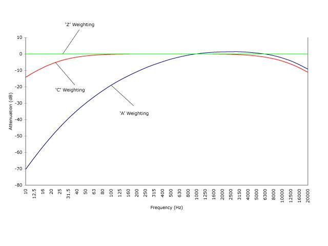
Another aspect of stimulus presentation that is often ignored involves the method by which we measure stimulus intensity.  Standard decibel (dB) meters that one might buy at your local electronics store or hardware store are known to measure the intensity of sound.  However, most individuals are unaware that the decibel measurements output by these meters are adjusted depending on their frequency.  We can see this in the plot below:

The weightings applied to commercial dB meters are designed to comply with OSHA standards so that acoustic hazards in work environments can be detected. Unfortunately, this means that the commonly available detectors are optimized/weighted for human hearing.  Thus, is is best to use a C or Z weighting on a decibel meter in order to obtain a more absolute measure of dBs and then to manually correct the volume to ensure that it is well above the auditory threshold for the rodent at that frequency.

All in all, being aware of these factors allows you to choose proper stimuli, assess stimuli effectively, or make adjustments to stimuli when necessary to ensure experimental reliability.  Similar concerns arise when considering any other sensory stimulus.  So, without a doubt, you need to be aware of the limitations of the species you are working with.

D.J. Barker

Perfusion/Fixation

A video on how to perform a perfusion by Gage et al. (2012)

This is a well conceived video on perfusion. It is important to note that the apparatus for perfusing buffers and paraformaldehyde differs from lab to lab. Still, the procedure described in this video is very sound and well described. Given the widespread use of perfusions in research, any researcher would do well to read about the principles behind the technique. Those interested should pursue other resources to learn more about the procedure.

Some relevant questions you might want to answer for yourself:

--What precautions must be taken when handling the chemicals used in this process?
--Why is paraformaldehyde used instead of formalin for immunohistochemistry?
--What is Sodium Azide? Why is it used? Are there any disadvantages to using sodium Azide?
--What is being preserved using this method? What is not being preserved?
--Name a few alternative approaches to retrieving neural tissue
--What is a good rule of thumb for the amount of fluid needed to pass through the body during a perfusion?


D.J. Barker

Renaming files in Matlab

A nice trick for renaming large numbers of files in Matlab:

Using Java code to rename files in Matlab

Correcting for Familywise Error

When conducting a group of statistical comparisons, it is important to understand the concept of familywise error or the 'familywise error rate'. The concept of familywise error describes the probability of incorrectly rejecting the null hypothesis. Perhaps more informally, familywise error represents the odds of reporting a statistical difference when no such difference exists.

 To understand why familywise error is important we must revert back to concepts learned in a basic introductory statistics class. First, we generally compare t-values (or other test statistics) to a known distribution of scores (t-scores in this case). Like any distribution, some values near the center of the distribution are more likely to occur than others. By understanding the odds that a given t-score will occur, we are then able to designate values that define regions of the distribution that are unlikely to occur as "critical values". That is, values above or below these critical values only occur with a certain limited probability.

 The exact probability we choose to define the critical values is arbitrary and often driven by tradition. As mentioned previously, we want to select values that are unlikely to occur in order to reliably report statistical differences. On the other hand, selecting values that are too stringent might cause us to report that no difference between our samples exists when in fact a difference does in fact exist. In psychology, a alpha of 0.05 is generally designated and denotes that falsely rejecting the null hypothesis should only occur 5% of the time. This value has been shown to provide a nice balance between selectivity and reliability.

Having said this, it is important to realize that the probability of finding a test statistic that is outside of the critical values for a single comparison is 1 in 20 (5%).  However, we also know from probability that the more chances one has, the more likely an event becomes. For example, if a player's chances of winning the lottery with one ticket are 1 in 14 million,  that player can increase his chances to 1 in 14,000. As you might imagine, this presents a problem when running multiple statistical comparisons.  The more statistical tests we run, the more likely it is that we will incorrectly identify a statistical difference (i.e. incorrectly reject the null hypothesis).

There are many ways to correct for this problem. Each different correction has its pros and cons and each correction may be more or less stringent than the next. Thus, one must consider how conservative of a correction a given situation calls for, if a desired correction will be overly liberal or conservative given the number of comparisons being made, and perhaps if the number of comparisons being made even warrants a correction at all.

One common correction that you might use is a Sidak correction.  This is a simple correction to calculate using the following formula:

 1−(1−α)^(1/n)

where, α represents your chosen alpha level and 'n' represents the number of comparisons being made.  This formula returns a corrected p-value that should be utilized in in lieu of alpha for each of your multiple comparisons when deciding whether or not to reject the null hypothesis. For example, if one were to make five separate statistical comparisons, the Sidak correction would dictate that only p-values of < 0.01 should be considered instead of the typical p< 0.05.

Try utilizing the formula yourself to calculate a corrected p-value and see how increasing the number of comparisons necessitates a greater correction.

D.J. Barker

Gas Chromatography explained

After our discussion today, I went looking for some tools to help illustrate the process for gas chromatography. Below you will find a schematic of the GC equipment and a great video by thermo scientific  demonstrating how a column works.

Techniques in Neuroscience

For those interested in a crash course in neuroscience techniques, I would highly recommend the book entitled Guide to Research Techniques in Neuroscience. I recently purchased this book and have been examining it most of the evening.  Techniques covered in the book include, but are not limited to:

-Imaging
-Animal Behavior
-Stereotaxic Surgery
-Electrophysiology
-Microscopy
-Genetics

This book will not necessarily give you the necessary skills to perform the techniques listed, but will give you a well-rounded overview of the techniques that might allow you to more effectively read, critique, and effectively discuss studies with techniques that are outside your purview. More importantly, this book provides a good middle ground between typical texts that are either oversimplified, overly-technical, or disconnected from the "hands on" side of neuroscience.

    D.J. Barker

How to Shape Behavior

In behavioral experiments, training animals to reliably perform the task is crucial to the success of the task. Still, finding ways to produce behaviors--no matter how simple--can prove challenging for any research scientist. Not to worry. Teaching animals to perform a desired behavior can be accomplished through a process called "shaping".  More specifically, shaping is a method for conditioning a behavior and was first introduced by B.F. Skinner.  The procedure involved gradually  changing behavior over time until a certain target behavior is reached.

This brings us to our first "rule" of shaping: Learning is a gradual process. This means that shaping a new behavior involves patience. One technique used to "patiently" shape behavior involves "successive approximations" of the target behavior.  The use of successive approximations involves reinforcing behaviors that come close to the target response without necessitating that a subject actually emit the target behavior.

One example of shaping might involve teaching a child to write his or her name. This might first involve praising the child only for correctly forming the first letter.  Eventually, in order to reach the goal of having he child write his/her full name, it becomes necessary to raise the bar until the child has written the second, third, and eventually all of the letters in the name. Importantly, successive approximations also allow for failure by only raising the bar a little at a time. Thus, the second rule of shaping is that learning involves making mistakes.  Certainly, it is just as important for an individual to learn what NOT to do as it for them to learn the desired behavior. To continue with the above mentioned example, it might be important for a child confusing the letters "M" and "N" to correctly learn to discriminate these letters in order to correctly spell his/her name.

A third rule of shaping is that reinforcement must be given in a consistent, steadfast manner.  When reinforcing approximations of a target behavior, it is important never to lower the bar once a behavior that is more proximal to the goal behavior has been learned. For example, it would not be effective to reward a child who had learned to spell half of their name for only inscribing the first letter. On the other hand, one must also be careful not to raise the bar too quickly. It is important to consistently reinforce each "step" in the approximation process for long enough to ensure that the subject has mastered the behavior before moving on.

The last major rule for shaping is that an experimenter must learn to observe behavior. To most rapidly shape an animal, an experimenter must exploit innate behaviors exhibited by that animal.  Realistically, an experimenter should take a naturally occurring behavior that best approximates the target behavior and begin to reinforce that behavior as an initial approximation. To do this, an experimenter MUST observe and understand an individual's behavior. The key word here is "individual", as no two animals will be shaped in the same manner. Thus, to shape a specific individual, one needs to have a well-developed understanding of the behavioral repertoire that an individual possesses. 

Shaping a lever response in an highly mobile rat might involve reinforcing moments when the rat's innate ambulations place the animal in close proximity to the lever. Once the animal has learned that the quadrant proximal to the response manipulandum is special, it would be easy to begin raising the bar and better approximating a lever response.  In contrast, a scared animal that freezes in the corner of the chamber could not be shaped using this same method (at least not easily).  As you might imagine, shaping this animal would necessitate a very different strategy.  One such strategy might be to spread pieces of food around the chamber so that our scared rat begins moving around to eat the food and better approximating our more mobile rat. 

Lastly, it is important to realize is that shaping takes practice. Practice allows you to observe animals behaviors, develop an understanding of individual differences among animals, and to develop a plan in your head for how to carry out your shaping procedure. Each subject is different, and each task we might ask a subject to complete comes with new challenges. Still, despite all of these differences, the essence of shaping never really changes. Happy shaping!

        David Barker

Intro to SigmaPlot

For those with experience in Microsoft Excel, SigmaPlot will be a fairly intuitive program to use.  Still, the program does present some challenges as you try to customize graphs and can take a little getting used to.

When opening SigmaPlot, you are first presented with a spreadsheet.  To begin graphing, one should copy and paste relevant data into the spreadsheet.  Generally, it is best to have each series of data in a given column.

Once the data have been inserted, you can choose among the different graph types using the icons on the left hand side of the SigmaPlot window.  It is generally worth exploring the available options, as each plot has its own unique characteristics. For example, one plot may allow for a single series of data while another might allow for multiple series.

Once you have selected a plot, follow the prompts to select your data. For the above example we have chosen a "Simple Line & Scatter-[with] Error Bars". We will use this to plot the average body weight of rats across days of an experiment. Having selected our graph, we designate in the first menu that our data are arranged in columns and then (for this example) can select either that we have "XY pairs" or a "Single Y" in the subsequent menu.  Given that our X-axis consists of incrementing integers (number of days), we can select Single Y and allow SigmaPlot to fill in the integers for each day (1-21) or we can select XY pairs and use a column we have filled with numbers 1-21 (col 1, above).  Finally, as described in the sigma plot menu, we will use the mouse to select columns corresponding to our X series (if XY pairs), Y series, and Error terms. Click "finish". Congratulations! You have made your first graph.

To make most changes to the graph, one can right click on the graph and choose "graph properties". This allows you to change an array of properties including the symbol types, error bar style, line style, or scaling of the X and Y axes. Most of these values can be adjusted using the user interface by adjusting the provided slider bars or changing the values in an input box.

For those that are new to SigmaPlot, exploring these menus is one of the most beneficial things you can do.  For practice , you might take a very simple graph and plot is with a number of different settings.  As a careful scientists, you would do best to change one thing at a time so that you can see your changes take effect.

It should also be stated that properties of the plot can sometimes changed by using your mouse to select a specific part of the graph. This can be done to edit text for things like the axis labels by simply clicking on these items and typing in the new lab. Similarly, you can edit other properties of items (e.g. the color of text or lines) by right clicking that particular item, and selecting the properties for that specific item (e.g.,"text properties" for the Y axis labels). Selecting individual items in this way can also be used to delete specific components of the graph, move certain items, etc.

One final problem we will explore is how to use text for the tick labels on an axis. To do this, you first need a column filled with strings (text) that represent your data.  For the current example, we will use 21 letters of the alphabet in place of day numbers.  Once we have a column with letters A-U (C), we enter the graph properties (See above), select the axes tab, and click the "Tick Label" icon in the left-hand menu (A). Under the top pull down menu (type), select the column number containing your axis labels. Next, you may need to enter the left-hand menu for "Ticks" (A) to change the tick interval to "Manual" (B) and select the number corresponding to the desired tick interval (every X data points starting at Y).

NOTE: One quirk of SigmaPlot is that it often applies labels that include strings such that they do not line up with your data points.  This can easily be fixed by inserting a blank cell before or after the cells containing your labels in order to line the correct label up with the correct data (Notice the blank cell at C, above which changes the labels from #'s 0-20 to #'s 1-21).

Now that you have an introduction to SigmaPlot, you can begin learning how to perform more advanced tasks.  You can find some other SigmaPlot tricks here, or you can start playing around with the things you learned today.  Happy Graphing!

    David Barker

My final graph after doing a little playing: